Wild things, part 5

On one level, what Richard Taylor was asking for was easy. Below is an example of blurring an image. On the left is the original, and on the right is the blurred version.

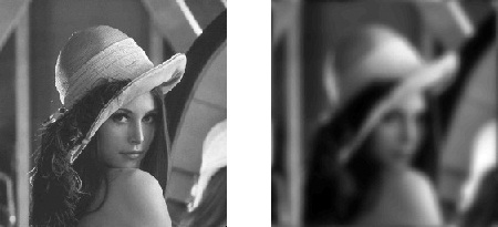
By the way, for those of you who don’t know, this is an image of Lena Sjööblom. She was originally the Playboy playmate of the month in November 1972. Her image started to be used by appreciative computer vision researchers at the University of Southern California, and she ended up becoming the standard test picture for image processing research. Needless to say, the original photo showed quite a bit more of Lena. If they had used the entire image, the field of image processing might have taken quite a different turn. You can read the whole story here.

Blurring is easy when you use a camera. Just push the lens out of focus, and you get a nice blurry image. That’s because every point of the original image gets smeared out over many points of the resulting blurry image. I could have done it that way in computer software, but that would have taken a very long time. Computers then were a lot slower than they are now. The image below shows the problem I was facing:

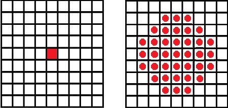
If you want to blur an image, then every pixel of the original image (left) needs to get added to many pixels of the blurred image (right). This is a serious problem if you’re image is typical size – say 1000 × 1000, or a million pixels. If your blur size is 30 × 30 pixels, then every pixel in the original image needs to get added to about 1000 pixels in the blurred image. We’re talking about a billion or so operations here. Back when we were doing the Wild Things test, that was way too much computation to be practical.

I needed to come up with something faster. The breakthrough came when I had the idea of smearing. If you think of the value at one pixel of an image, you can do the following to smear that pixel value out in a horizontal direction. First, copy the pixel value to another image, but offset to the left. Also copy the negative of the pixel value to this other image, but offset to the right. You can see this represented in the image below, in the transition from A to B:

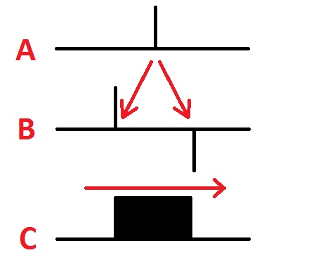
Now here comes the secret sauce. Sum up all of the values in the result, starting from the left and going all the way to the right. What you end up with is the pattern in C above – a smearing out of this one pixel value over an entire region. What’s cool about this is that it doesn’t matter how far apart you separate the positive and negative values – the amount of computation stays the same.

Of course it’s not all that useful to blur out a single pixel. But the nice thing is that if you start with more than one pixel value, everything still works. In the image below we have two non-zero pixels. Applying the same trick (going from A to B in the image), we get some positive values and some negative values. If we sum everything up from left to right (going from B to C) we end up with a blurred version of the original.

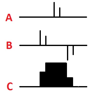
This trick works no matter how many pixels you start with in the original image. In fact, you can start with any image at all, apply the same trick, and you end up with a smeared out version of your original image. And the amount of computation doesn’t increase as the smearing gets bigger.

This gave me a way to create nicely blurred images without requiring too much computation. I could just do this smearing trick twice in the horizontal direction, and twice in the vertical direction, and end up with a really nicely blurred image – without needing to wait too long for the result.

So how did this little fast blurring trick let me create images of Max and his dog that looked rounded and 3D? We’ll get to that tomorrow.