Month: January 2025

What if there is some sort of fundamental difference in the way that people think in different parts of the world? I don’t mean a psychological difference, but more of a metaphysical difference.

Maybe there is some deep division in world view, in what we think of as rightfully animated, and as unrightfully animate.

It is possible that when we approach matters that seem as rational as technology, we bring with us values that are much deeper and more primal — not values that come from scientific thought, but rather values that come from metaphysical viewpoint.

There is a lot to unpack here. More tomorrow.

There was a time when I was doing a lot of research on procedural charaacter animation. That research included simulation of the emotional nuances of both body language and facial expression.

People always seemd very interested in this work. But then I would talk about the possibilies of applying these technologies to robots, and then I would get a very different reaction.

As soon as we started discussing robots showing emotion, my listeners began to make associations with Frankenstein. Machines that imitate human feelings appeared to hit a raw nerve, and people would become genuinely concerned.

But then I gave a talk in Japan, and I found that attitudes were completely different. When I gave talks there about procedural character animation, audience members would ask about whether the results could be applied to robots.

Clearly there is something going on here. More tomorrow.

I recently went to a little dinner party at a friend’s house, and was introduced to the wonderful game of Rummikub. It’s a game for 6-8 players, but I enjoyed it so much that I also wanted to be able to practice it on my own, wherever I happened to be.

While I don’t carry a set of Rummikub tiles around with me everywhere, I do carry my MacBook. So the other day I implemented a sort of practice solitaire version, just for fun.

It’s not the same as playing with other people. For one thing, you don’t get that thrilling uncertainty of wondering what moves other people will make during their turn.

But I find it to be quite meditative and enjoyable. When you play it, you’re basically solving fun little puzzles.

But why take my word for it? You can try it out for yourself HERE.

As long as I am using my new implementation of 3D noise to build something as lofty as clouds, I thought another good test would be to try the opposite. And the opposite of the heavens is the earth. So today I made a rock.

The rock is built by creating a sphere, and varying the radius of the sphere via a fractal sum of noise. That is, I displace the surface of the sphere by adding together noise at many different scales.

This is pretty much what you see when you look at mountains or coastlines. Something that would otherwise be straight has been perturbed by random forces at many different scales. And 3D noise is really good for simulating that.

For good measure, I added a subtle mottling to the surface color, to suggest that the rock is a composite of various minerals. You can see the result below.

One thing that makes me happy about modern GPUs is just how darned fast they are. I find that I can create procedural textures with multiple calls to my noise function at every pixel, and the GPU keeps up just fine.

For example, click on the image below to see a live simulation of roiling clouds. When you follow the link, you can also see the complete vertex and fragment shader code that generated the simulation.

This cloudy skies simulation was created by calling 3D noise multiple times at different scales. I find that I can call noise up to 8 times per pixel and still maintain a steady frame rate of 60 frames per second on my phone.

Let’s work out some numbers. The simulation itself is 1000×1000, so that’s one million pixels.

My noise implementation calls the cosine function 4 times to compute a repeatable random number. So to evaluate noise once, that’s 4 cosine functions for each of the x,y,z axes at the 8 corners of a cube.

That’s 4x3x8 = 96 cosine computations. Multiply that by 8 calls to the noise function per pixel, then again by one million pixels, and then again by 60 frames per second.

The result? More than 46 billion calls to the cosine function every second — not counting all the other computations involved. And it all runs just fine on the low power GPU of a smartphone.

Pretty cool, yes?

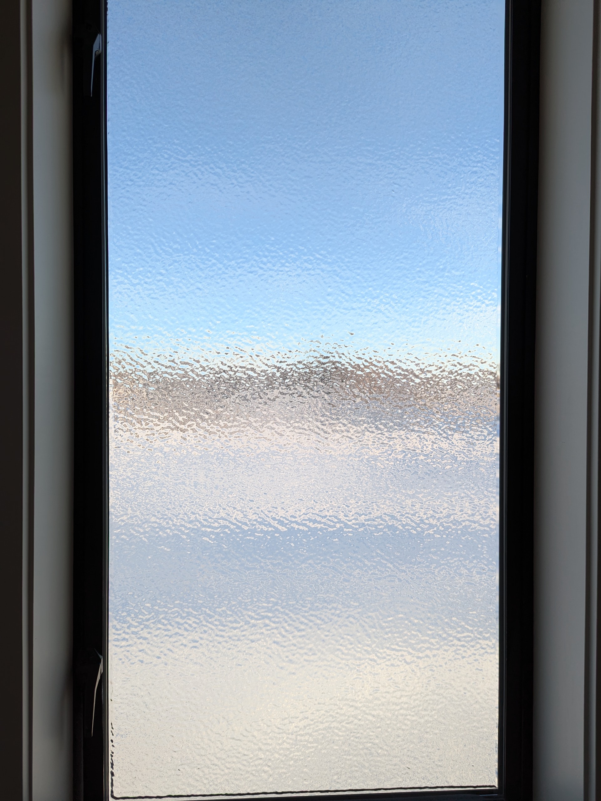
After yesterday’s big winter storm, this morning I awoke to find the windows covered in ice. I took some photos.

Below left is a photo of one of the windows here. To its right is a close-up photo of the same window.

The reason for this texture is that ice has lower density than water. That is why ice floats.

The colder water toward the outside of the window freezes first, and therefore expands faster. This makes the outside surface area increase, causing the surface to buckle.

The result is a random bumpy topography. Because of the underlying physics, all of the bumps, although randomly placed, are about the same size.

It is similar to the process — a gradual increase in surface area over time — which causes drying paint to develop a bumpy surface, with all of the bumps being about the same size. And this particular natural phenomenon was also my original inspiration for creating synthetic band-limited noise, all those years ago.

For the last several days I have been writing posts about noise. So it seemed like a wonderful coincidence, when I woke up this morning, to see something like this.

It was as though nature itself was sending me noise.

Or maybe it was sending me a signal.

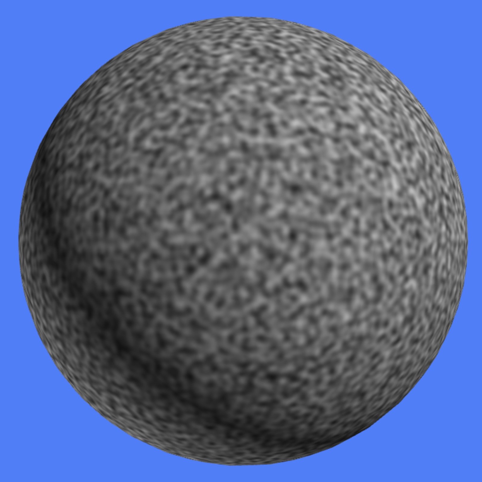
One of the first things I like to do when I implement any procedural texture is slap it onto a sphere, and then rotate the sphere. That’s a pretty surefire way to find out whether there are any unwanted patterns, repetitions, or other objectionable visual artifacts.

So I did just that with my latest implementation of 3D noise. Fortunately, it looks as though this particular implementation passes the rotating sphere test.

To link to the result and see for yourself, you can click on the image below.

More tomorrow.

The language, architecture and even general philosophy of a CPU and a GPU are radically different, so it is intriguing to see them performing the same task. Here, two wildly different kinds of computers are producing exactly the same result.

To anyone looking at the two images below, they seem to be the same. But a programmer reading the corresponding code will see two clearly distinct programs.

In one case, the program is optimizing for the massive parallel pipeline capability of a GPU. In the other case, the program relies on the flexibility of programming in Javascript on a CPU. For example, on the CPU there is no built in normalize function to set a vector length to one. But it takes just a single line of Javascript code to derive such a function from a dot product:

let normalize=v=>(s=>v.map(a=>a/s))(Math.sqrt(dot(v,v)));
From the perspective of a computer graphics designer, having the same noise function on both the CPU and GPU means that the designer is free to go back and forth between the two environments when creating noise-based models. You can choose to implement one part of your design to run on the CPU and another part to run on the GPU, and the results will match.

More tomorrow.

For years I have been wanting to implement a version of my 3D noise function that produces the same result on the CPU and GPU. But I also wanted it to do other things as well:

(1) It needs to use only standard WebGL and Javascript
(2) It can’t require loading any data tables
(3) It must run insanely fast — even on my phone

Well, I finally got around to it. I’ve posted a little side by side test of the GPU and CPU implementations, together with the source code for each.

The test shows an X,Y slice of 3D noise traveling in Z over time. You can see it here.

The comments on yesterday’s post remind me of an experience I had some years ago. I was at a conference in Germany, and one of my colleagues took me to where Carl Friedrich Gauss had once lived.

My colleague and I had both heard the story of how the world first learned that Gauss was a mathematical genius. When he was a child in school, his teacher gave the class an exercise to keep them busy.

In those days, every student had a slate and a piece of chalk to write with. The teacher told them to add up the numbers from one to one hundred.

While all the other children toiled away at the task, young Gauss simply wrote a number down on his slate and then set it down. The teacher asked him why he was just sitting there.

Gauss showed his teacher the slate, which had the proper sum on it. The boy had figured out the formula in his head, had solved it, and had written down the proper answer.

We then discussed whether that was actually a true story. “What are the odds”, my colleague asked, “that the story is real?”

Never in my life have I been fed a better straight line. “I would say — fifty fifty.”